
Excel Worksheet Functions
=Match(lookup_value, lookup_array, [match_type])
MATCH finds the location of a value in a specific row or column.
- MATCH searches a row or column for the lookup_value.
- It returns the cell location at the row OR column where the lookup value is found.
- By itself, MATCH isn ' t terribly useful since MATCH only returns the cell location, not the cell value.
- When combined with other functions, such as INDEX, it can be used to get around some of the limitations of VLOOKUP or HLOOKUP.
SYNTAX: =Match(lookup_value, lookup_array, [match_type])
| Lookup_Value | This is the value you want to find. This can be a number, text, a cell reference, or a logical value. |
| Lookup_Array | This is a row or column where the match will be found. The lookup_array must be a single row or column. |
| Match_Type |
0 = Find an exact match 1 = Closest value that is less than or equal to the lookup_value Lookup_array must be in ascending order 2 = Closest value that is greater than or equal to the look-up value Lookup_array must be in descending order |
Example:
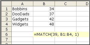
=MATCH(39, B1:B4, 1)
- Look in the lookup_array of B1:B4 for the value 39.
- The match_type value is 1, which means it will find the exact number or the closest number that is less than 39.
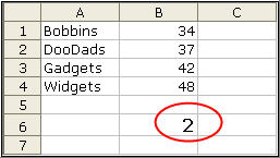
- The number 2 is returned by the MATCH formula because 37 is the second element in the lookup_array.
Example:
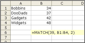
=MATCH(39, B1:B4, 2)
- Look in the lookup_array of B1:B4 for the value 39.
- The match_type value is 2, which will find the exact number or the closest number that is greater than 39.
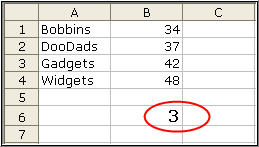
- The number 3 is returned by the MATCH formula because 42 is the third element in the lookup_array.
Example:
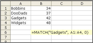
=MATCH("Gadgets", A1:A4, 0)
* Look in the lookup_array of A1:A4 for the value Gadgets.
* The match_type value is 0, which means to find the exact match.
* The text in cell A3 is an exact match.
* The value 3 is returned by the MATCH formula because Gadget is the third element in the lookup_array.
Copyright © 2006-2019, LQSystems,Inc. All rights reserved.