VLookUp Function

by Linda Quinn

Close Window Print Page

=VLookup( Lookup_Value, Table_Range, Column_Number, [Approx or Exact])

VLOOKUP finds the data in a specific row and column within a table of data.

It looks for a given value in the first column of the table and then retrieves
values from other columns in the same row.

Lookup Value	The value being looked-up. This can be a value, a cell reference, or text.
Table Range	The table that contains the look-up values. VLOOKUP always looks in the leftmost column of the table for a value that matches the Lookup_Value The Table_Range can be an absolute cell reference or a named range.
Column_Number	The column containing the value to be returned. This is the number of columns to the right in the Table_Range. The result will be in this column at the same row where the lookup value was found.
Approx or Exact Match [OPTIONAL]	If FALSE , an exact match must be found. If TRUE , the closest match (less than the lookup_value) is selected. Data must be in order if TRUE* is selected.*

EXAMPLE:

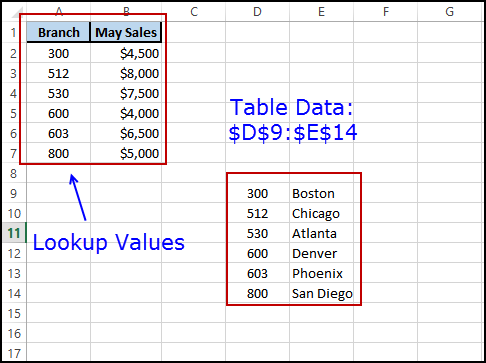
Here is a list of Branch Numbers with their May Sales Numbers:

We want to put the appropriate Branch Name in column C .

Notice that there is a table of branch numbers with their names at the range D9:E14 .

vlookup

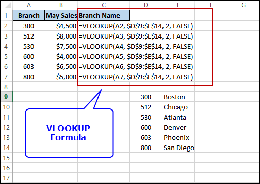
In column C row 2 we can place the following lookup formula:

=VLookup(A2, $D$9:$E$14, 2, FALSE)

The lookup values are the values A2, A3, etc. These reference the values being "looked up"
Notice the dollar signs around the D9:E14 table_range. This is an absolute reference to the branch name table range. The table will always be in this location.

We could assign a name to the range $D$9:$E$14. If we named it "Branch" then the formula would be

=VLookup(A2, Branch, 2, FALSE)

vlookup

The results are displayed below:

vlookup

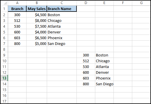
Here ' what happened:

In this example, the value in A1 , which is 300 , is looked up in the leftmost column of the range D8:E12 .

300 is found in D8 .

In column 2 of the found row of the table range, which is E8 , is the value Boston .

This is the value that will appear in cell C1

.

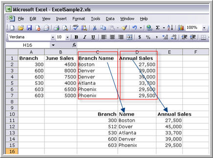
Another Example - Multiple Lookups of the Same Table-Array

In this example, we have the branch numbers and the June sales amounts in columns A and B .

The lookup table has a third column that contains the annual sales for each branch. [E10:E15]

vlookup

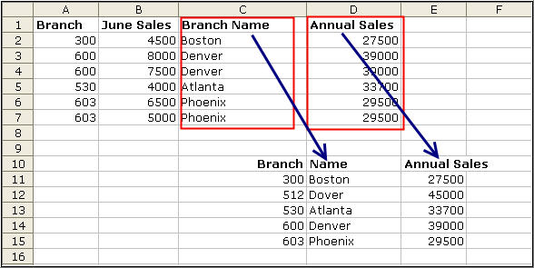
Create a Vlookup formula in column C. (=VLOOKUP(A2, $C10:E15, 2) .

This formula will search the leftmost column of the table range ($C$10:$E$15) for the value in A2 (300) .

When the value 300 (A2) is found at row 11, the formula will look in the second 2 column of the table to get the branch name.

In column D, create a similar formula except the column number will be 3 instead of 2 because we want the annual sales for the selected branch.

(=VLOOKUP(A2, $C10:E15, 3)

The results of the formulas are shown below:

vlookup